4. Examples
This section will provide you with selected examples on how to setup AGX related content in Unity 3D, focusing on the practical side of creating your own virtual physics assets.
To follow along the examples, download the example assets corresponding to the example you want to learn using the example window.
4.1. Manually installing example packages
While using the example window is the preferred approach for installing examples, it is sometimes desirable to install the examples directly through a .unitypackage file. These files are available for download using the link at the start of each example section.
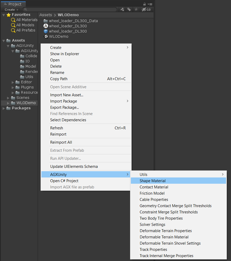
Since many of the machines used in the examples are shared across multiple examples, these are packaged separately and are distributed as NPM packages which can be installed via the Unity package manager (UPM). This requires the project to configure a Scoped Registry to find the machine dependencies when downloading an example.
To do this, open the Package Manager project settings (Edit -> Project Settings -> Package Manager)
and add a new scoped registry with the following configuration:
Name |
AGXUnity Registry |
URL |
|
Scope(s) |
com.algoryx.agxunity.machines |
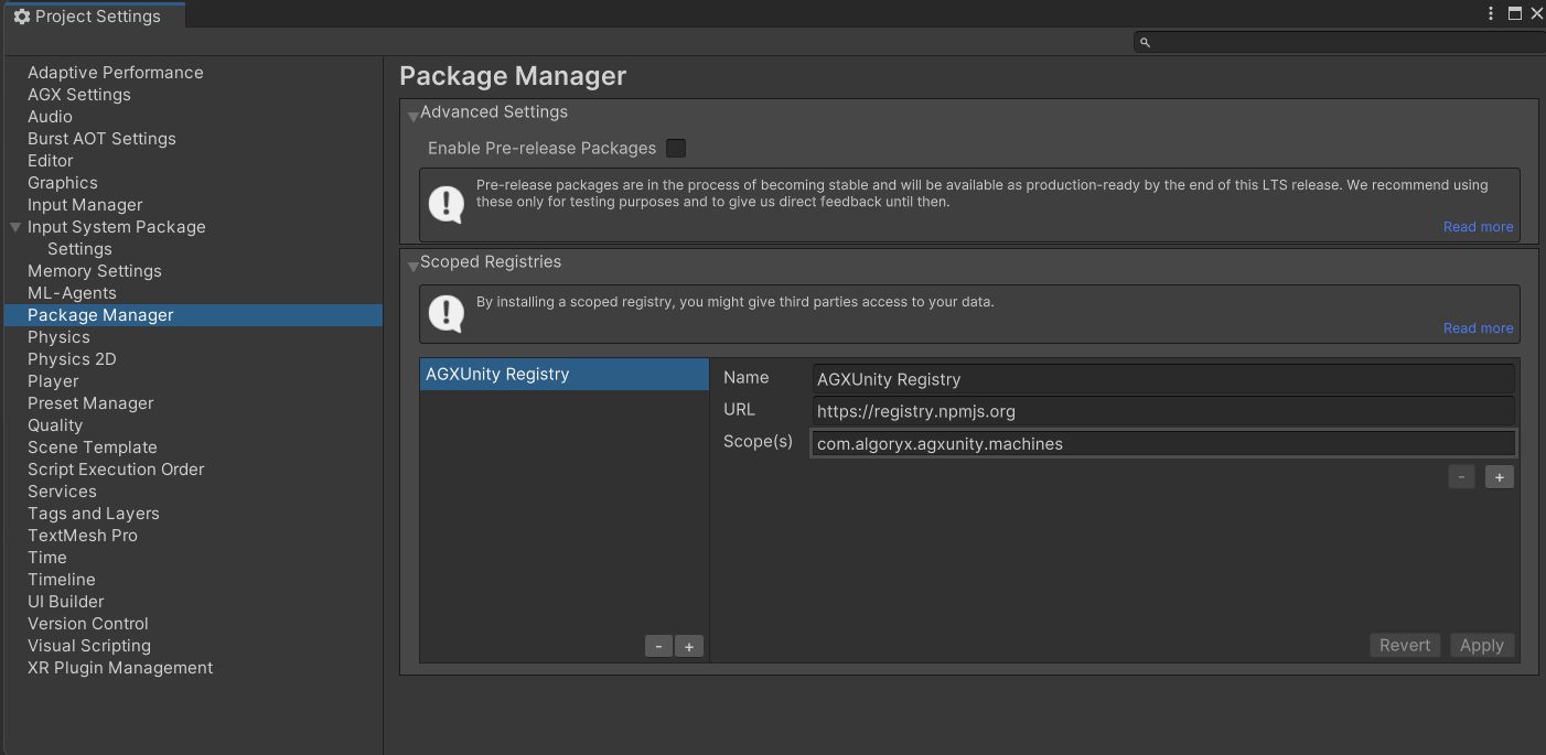
The Package Manager window after adding the required Scoped Registry.
After adding the scoped registry, each machine can be downloaded through the Package Manager
(Window -> Package Manager) and selecting the My Registries package source.
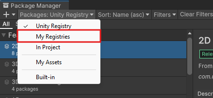
Selecting the My Registries package source in the package manager.
4.2. Fixing invalid materials for machines
If the material for a machine is broken when importing, the cause is likely one of two depending on the AGXUnity version used.
For machine package versions < 1.1.0, the materials used were the Built-in standard material. Since the packages are readonly,
there is no easy way to upgrade these when using HDRP or URP, causing broken materials. A workaround for this was added in AGXUnity 5.3.0
and machine packages 1.1.0. If HDRP/URP is used, the solution is thus to upgrade AGXUnity to 5.3.0+ or to manually download the Required Shader.
Likewise, if the project is using AGXUnity 5.3.0, make sure that the machines downloaded use a version later than or equal to 1.1.0.
4.3. Examples Window
Examples, and their dependencies, can be downloaded and imported using the
examples window which can be opened by clicking AGXUnity -> Examples. An example
can be downloaded and imported when all dependent packages (such as Input System, ML-Agents), for the
given example, has been installed using the ![]() drop-down.
drop-down.
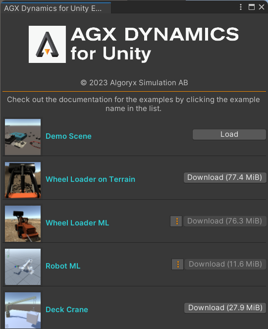
Examples window, open by clicking AGXUnity -> Examples.
Note
For versions prior to 5.2.0, the project needs to be set up manually to find the machine packages. For more information on how to do this, please refer to Manually installing example packages
4.4. Demo Scene
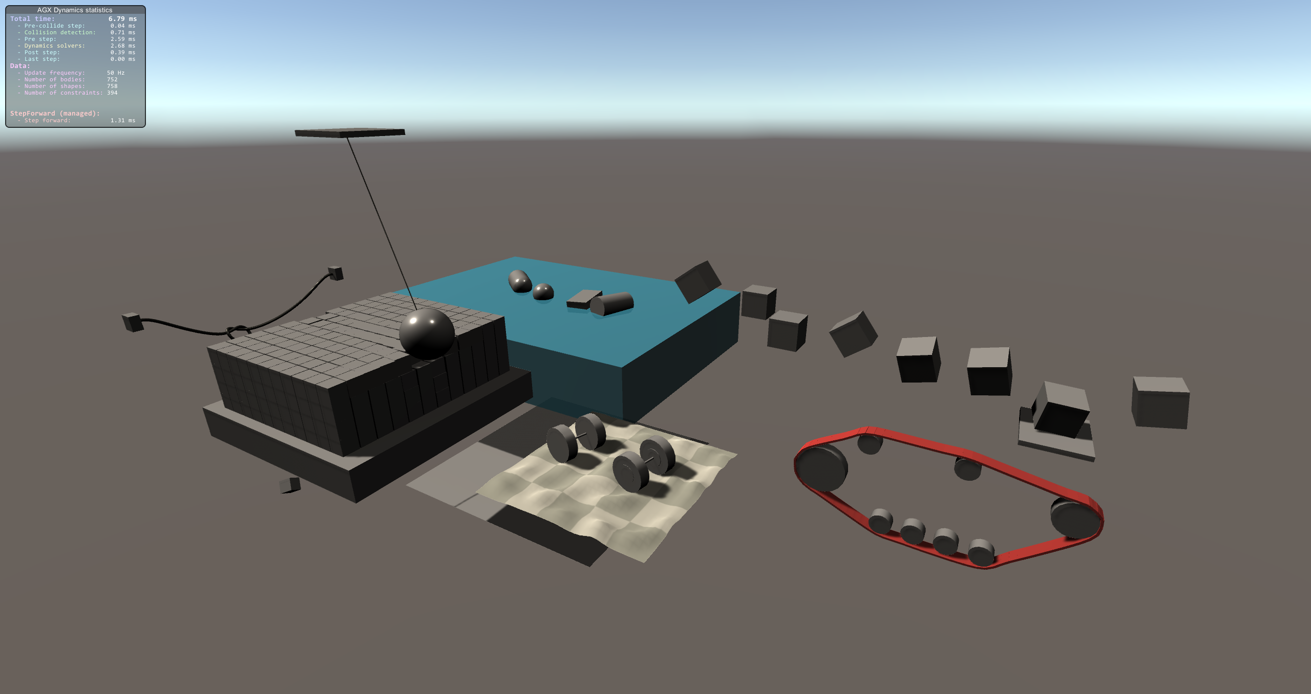
A demo scene showcasing various aspects of AGX Dynamics for Unity.
Note
AGX modules required to run example: Core, Cable, Tracks, Wire, Hydrodynamics, Tires, Sensor
Download this example as a standalone package: AGXUnity_Demo.unitypackage
This demo scene contains many of the features of AGX Dynamics for Unity, exemplifying how different parts may be configured.
The scene contains the following features:
4.4.1. Hydro- and Aerodynamics
4.4.2. Constraints
4.4.3. Tracks
4.4.4. One body and two bodies tires
4.4.5. Adaptive Model Order Reduction - AMOR and Wires
528 boxes that eventually will merge with the rotating, hinged, rigid body and some parts will split when the wrecking ball hits.
4.4.6. Cables
4.4.7. Cables
4.4.8. LiDAR
4.5. Wheel Loader on Terrain
Note
AGX modules required to run example: Core, Drivetrain, Terrain, Tires, Sensor
Download this example as a standalone package: AGXUnity_WheelLoaderTerrain.unitypackage
Here we set up a wheel loader on a Unity Terrain using the AGX Dynamics Deformable Terrain addon, which will let the vehicle dig and alter the terrain. We will be using the example wheel loader controllers provided by the AGX Unity package that shows off some basic ways of maneuvering a vehicle using input from keyboard or gamepad.
The Wheel loader model has been created in Algoryx Momentum and imported into AGXUnity as a prefab.
Note
Sometimes the Wheel Loader Input component doesn’t compile correctly together with the Input System package. We suggest starting the guide with the Input section to help prevent this, as shown below, and also to import the Input System package before you import the Example DL300 package linked above. See also the troubleshooting section in the bottom of this example.
4.5.1. Input
Note
Using the new Unity Input System requires version 2019.2.6 or later when
AGX Dynamics for Unity depends on the ENABLE_INPUT_SYSTEM define symbol.
The example controllers use the new Unity Input System package to allow for easy configuration of multiple input sources, in this case keyboard and gamepad. To use it, install it in the project using the Package Manager Unity window, which as of the time of writing this guide is still a preview package. The alternative is to use the legacy input manager as swown below.
4.5.1.1. [Optional] Legacy Input Manager
Using the old Unity InputManager, AGXUnity.Model.WheelLoaderInputController requires
some defined keys. The most straight forward approach is to copy the content below and replace
the already existing settings in ProjectSettings/InputManager.asset.
%YAML 1.1
%TAG !u! tag:unity3d.com,2011:
--- !u!13 &1
InputManager:
  m_ObjectHideFlags: 0
  serializedVersion: 2
  m_Axes:
  - serializedVersion: 3
    m_Name: jSteer
    descriptiveName:
    descriptiveNegativeName:
    negativeButton:
    positiveButton:
    altNegativeButton: left
    altPositiveButton: right
    gravity: 3
    dead: 0.3
    sensitivity: 1
    snap: 1
    invert: 0
    type: 2
    axis: 0
    joyNum: 0
  - serializedVersion: 3
    m_Name: kSteer
    descriptiveName:
    descriptiveNegativeName:
    negativeButton: left
    positiveButton: right
    altNegativeButton:
    altPositiveButton:
    gravity: 3
    dead: 0.001
    sensitivity: 2
    snap: 1
    invert: 0
    type: 0
    axis: 0
    joyNum: 0
  - serializedVersion: 3
    m_Name: jThrottle
    descriptiveName:
    descriptiveNegativeName:
    negativeButton:
    positiveButton:
    altNegativeButton:
    altPositiveButton:
    gravity: 3
    dead: 0.05
    sensitivity: 1
    snap: 0
    invert: 0
    type: 2
    axis: 9
    joyNum: 0
  - serializedVersion: 3
    m_Name: kThrottle
    descriptiveName:
    descriptiveNegativeName:
    negativeButton:
    positiveButton: up
    altNegativeButton:
    altPositiveButton:
    gravity: 3
    dead: 0.001
    sensitivity: 2
    snap: 0
    invert: 0
    type: 0
    axis: 0
    joyNum: 0
  - serializedVersion: 3
    m_Name: jBrake
    descriptiveName:
    descriptiveNegativeName:
    negativeButton:
    positiveButton:
    altNegativeButton:
    altPositiveButton:
    gravity: 3
    dead: 0.05
    sensitivity: 1
    snap: 0
    invert: 0
    type: 2
    axis: 8
    joyNum: 0
  - serializedVersion: 3
    m_Name: kBrake
    descriptiveName:
    descriptiveNegativeName:
    negativeButton:
    positiveButton: down
    altNegativeButton:
    altPositiveButton:
    gravity: 3
    dead: 0.001
    sensitivity: 2
    snap: 0
    invert: 0
    type: 0
    axis: 0
    joyNum: 0
  - serializedVersion: 3
    m_Name: jElevate
    descriptiveName:
    descriptiveNegativeName:
    negativeButton:
    positiveButton:
    altNegativeButton:
    altPositiveButton:
    gravity: 3
    dead: 0.3
    sensitivity: 1
    snap: 0
    invert: 1
    type: 2
    axis: 1
    joyNum: 0
  - serializedVersion: 3
    m_Name: kElevate
    descriptiveName:
    descriptiveNegativeName:
    negativeButton: s
    positiveButton: w
    altNegativeButton:
    altPositiveButton:
    gravity: 3
    dead: 0.001
    sensitivity: 1
    snap: 0
    invert: 0
    type: 0
    axis: 0
    joyNum: 0
  - serializedVersion: 3
    m_Name: jTilt
    descriptiveName:
    descriptiveNegativeName:
    negativeButton:
    positiveButton:
    altNegativeButton:
    altPositiveButton:
    gravity: 3
    dead: 0.3
    sensitivity: 1
    snap: 0
    invert: 0
    type: 2
    axis: 3
    joyNum: 0
  - serializedVersion: 3
    m_Name: kTilt
    descriptiveName:
    descriptiveNegativeName:
    negativeButton: a
    positiveButton: d
    altNegativeButton:
    altPositiveButton:
    gravity: 3
    dead: 0.001
    sensitivity: 1
    snap: 0
    invert: 0
    type: 0
    axis: 0
    joyNum: 0
4.5.2. Create the terrain
To quickly create a Unity Terrain with AGX Dynamics Deformable Terrain, we will use the top menu command AGXUnity -> Model -> Deformable Terrain as shown below.
Note
An AGX Deformable Terrain component could also be added through the “Add Component” on a game object, which might be suitable if modifying an existing terrain instead of starting from scratch.
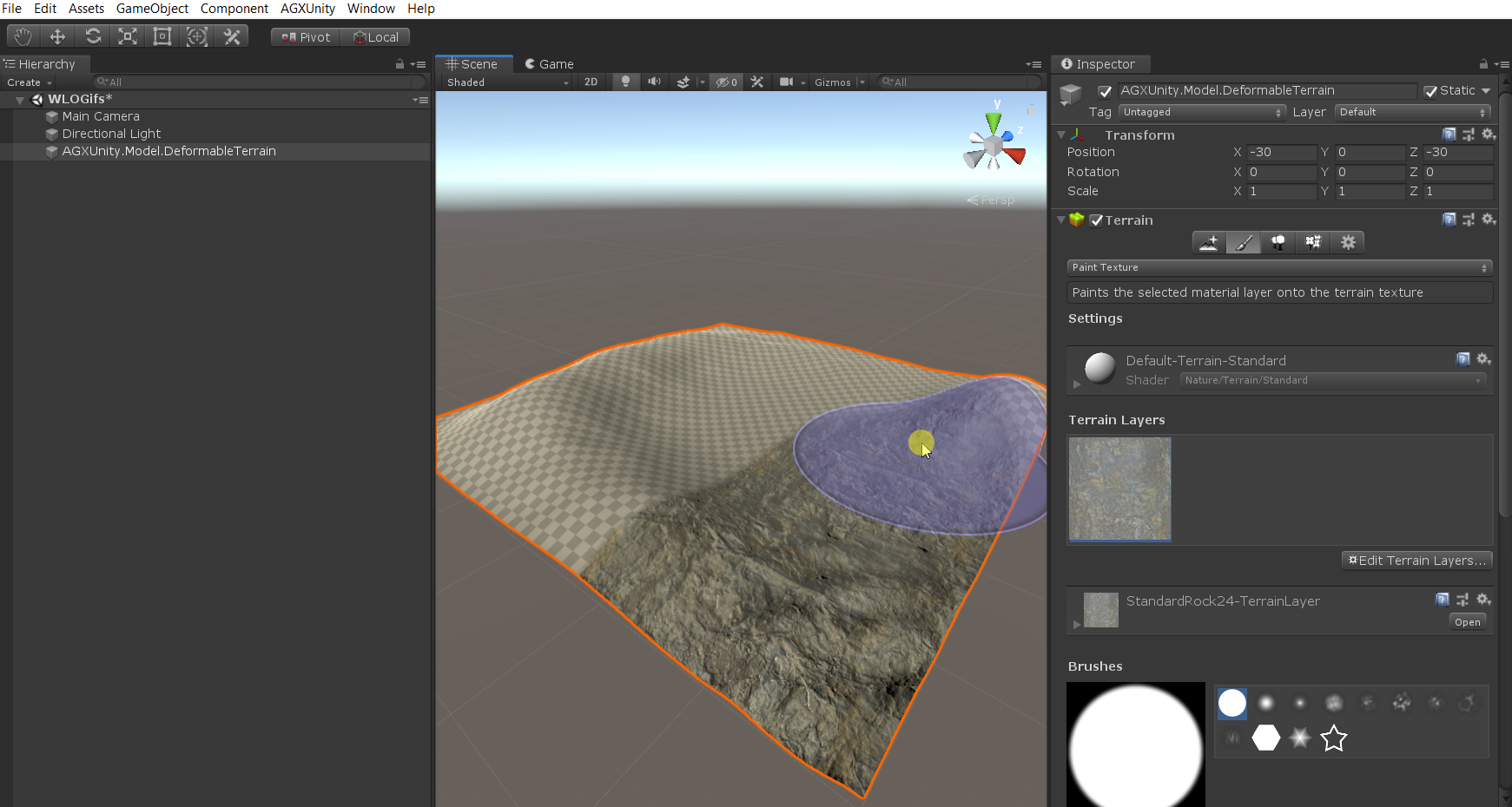
4.5.3. Modify and decorate the terrain
Next, use the Unity tools to modify the terrain to an interesting shape with varying heights, and optionally add and paint a terrain layer.
See also
Here we use the standard Unity3D terrain modeling features. For more details, see the Unity Terrain Tools documentation: https://docs.unity3d.com/Manual/com.unity.terrain-tools.html
4.5.4. Import the example Wheel Loader AGX model
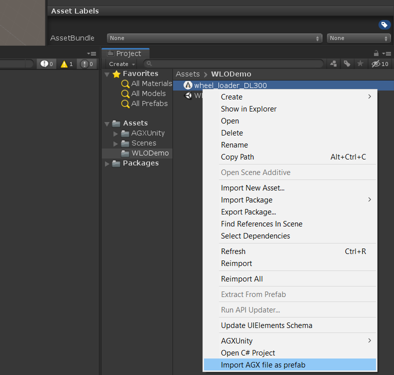
Objects to simulate in AGX can be created from basic shapes using Unity and AGX Unity tools, but it is recommended to use external tools for the creation of complex models. Here, we will import a .agx-file that contains visual meshes, constraints and rigid bodies already setup.
This is done by right clicking the file, selecting the menu option Import AGX file as prefab and then placing the prefab in the scene.
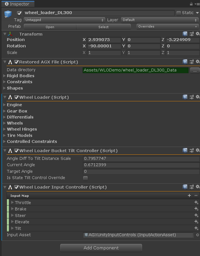
Included in the AGXUnity package are some example components to control and simulate a wheel loader. We will add these components to the newly created prefab by using the Add Component button on the prefab root object.
WheelLoader
WheelLoaderBucketTiltController
WheelLoaderInputController
4.5.5. Set up the shovel component
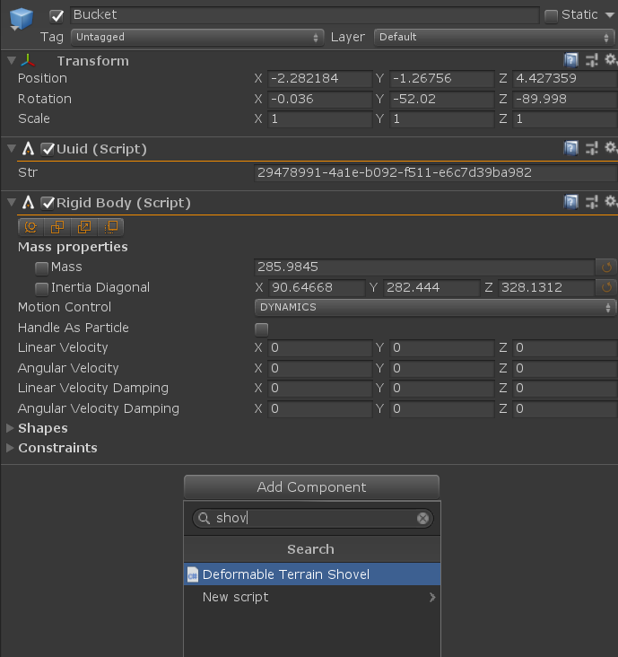
To give the wheel loader the ability to deform the terrain, we have to setup a Deformable Terrain Shovel component. To do this, select the RigidBody object corresponding to the bucket of the wheel loader.
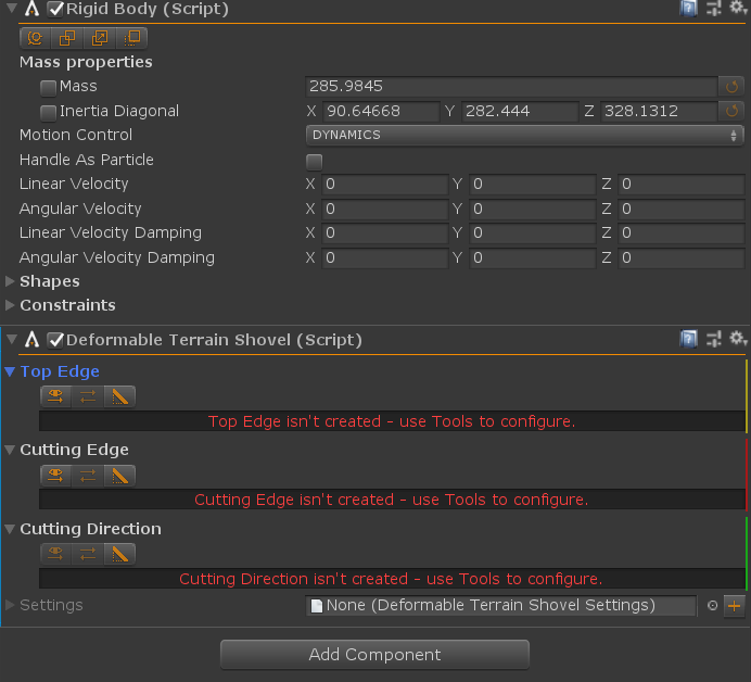
Next, we need to setup the shovel edges. Use the tools as shown below to set up the cutting edge, the top edge and the cutting direction.
4.5.6. Contact Materials
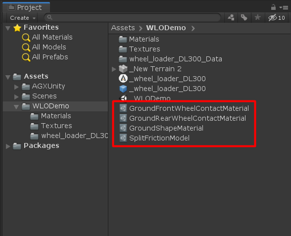
In order to adjust the friction between the ground and the wheels, we can specify a Contact Material. To do this, we will create a number of assets:
One ShapeMaterial-asset to represent the ground material
Two ContactMaterial-assets to represent the intersection between the ground material and the two front and rear wheel ShapeMaterials (predefined in the model)
A FrictionModel-asset to define the type of friction calculations used on the ContactMaterials
The below image shows one way of creating the assets and the created assets after renaming to suitable names.
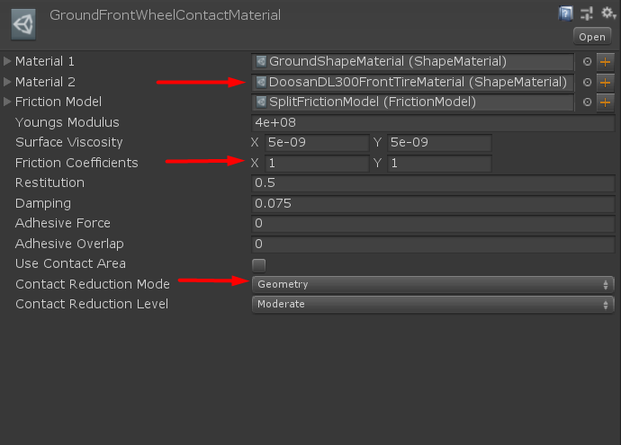
Next, we will set up the contact material to use the other assets as shown below. The wheel ShapeMaterial (DoosanDL300FrontTireMaterial and DoosanDL300RearTireMaterial) should be available in the menu by clicking the Select button to the right of the Material 2 field.
For wheel friction, Contact Reduction Mode can be used to provide a more stable simulation on uneven terrain with many points of contact (wheels), a high friction value (1) could also be used to simulate high grip - rubber on coarse gravel.
Now we will apply the new ShapeMaterial to the relevant AGX physical object, i.e. the ground. This is done by selecting the objects and dragging/dropping the shape materials from the asset list as shown below.
Finally, the two new contact materials need to be registered in the ContactMaterialManager in the scene, as shown below.
4.5.7. Deformable Terrain Particle Renderer
To visualize the soil particles as they are created, we will set up the DeformableTerrainParticleRenderer component. This is done by adding it to the the GameObject with the DeformableTerrain component, and setting a visual object (such as a basic sphere) as the visual to represent a soil particle. The visual should be an object in the scene, preferably hidden from the main camera view.
Here, we use the Unity way of creating a 3D sphere, remove the PhysX collider, move it out of view and assign it to the newly created particle renderer. A basic sphere will of course look not very interesting, so a model resembling a rock could be used instead, if available.
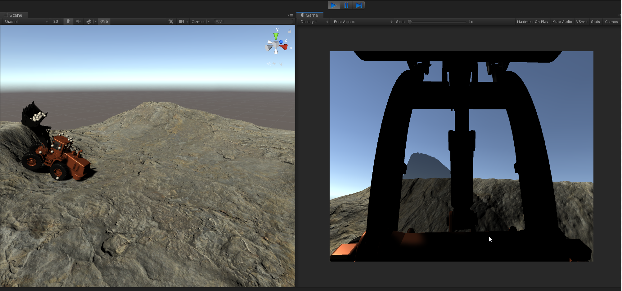
4.5.8. Test Drive
We’re good to go! Position the camera, start the simulation and use the keyboard to drive the wheel loader across the terrain, digging as you go! Some controls:
Drive / brake and turn: WASD keys
Raise/lower boom, tilt bucket: arrow keys
4.5.9. Auto-brake using LiDAR
The downloaded example package comes with a script called LiDAR Reverse Brake. This script reads LiDAR depth data and uses
it to automatically apply a braking force when there is an object closer than 1m behind the wheel loader and it is moving backwards.
This script is added to a new object under the RearBody along with an LiDAR sensor. In the example package, a pile of rocks
has also been added as an example of an obstacle to brake for.
For this example, the LiDAR is configured to scan in an arc in front of the sensor as to not hit the wheel loader itself. A rendering component is added to the object as well for visualizing the output points. This component is, however, not required for the auto-brake script to function.
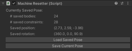
4.5.10. Resetting the machine to a saved location
The Machine Resetter script in the example provides sample code that can be used to save the current machine pose as well
as resetting the machine pose to the saved one. To do this, the script uses a combination of
agxUtil.jumpRequest
and agxUtil.ReconfigureRequest.
The initial pose of the Wheel Loader is saved on startup and can be saved during runtime using the T key or the button in the inspector.
The pose of the machine can be reset to the last saved pose using the R key or the button in the inspector.
4.5.11. Trouble Shooting
If you are using the Unity Input System package and nothing happens when you try to steer the vehicle, it is possible that the Wheel Loader Input Controller component is not functioning correctly. If working correctly, the component should look like this:
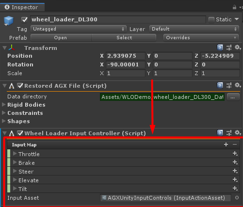
If it is not working correctly, it will probably look like this instead:
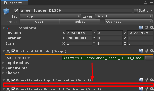
If your component looks like in the second example, you can try the following:
Remove the Input System package using the Package Manager
Reinstall the Input System package using the Package Manager
Select the Wheel Loader Input Controller component and assign the empty asset by using the button to the right of the empty field.
Hopefully this fixes the problem. If nothing works, you could as an alternative try the legacy input option outlined above.
4.6. ML-Agents Wheel Loader Way Point Controller
Note
AGX modules required to run example: Core, Drivetrain, Terrain, Tires
Download this example as a standalone package: AGXUnity_WheelLoaderML.unitypackage
Unity ML-Agents toolkit can be used to train autonomous agents using reinforcement learning with AGX Dynamics high fidelity physics. Realtime performance with small errors give the potential for sim2real transfer. This is a simple example how to setup the agent with observations, actions and reward together with AGXUnity. As well as, how you can step the ML-Agents environment together with the simulation and reset the scene after a completed episode. This agent controls a wheel loader to drive over uneven deformable terrain towards a list of way points. The ML-Agents documentation is a good resource for ML-Agents concepts.
In addition to AGXUnity you also must install ML-Agents. The Unity package is directly installed with the Unity package manager. That is enough for evaluating the pre-trained agent shipping with the example package. If you want to train your own agent you must install the ML-Agents python package. See the ML-Agents installation documentation for installation options. This example is trained using the versions:
com.unity.ml-agents (C#) v.1.3.0.
mlagents (Python) v0.19.0.
mlagents-envs (Python) v0.19.0.
Communicator (C#/Python) v1.0.0.
4.6.1. Create the Learning Environment
The learning environment is where an agent lives. It is a model of the surroundings that cannot be controlled but still may change as the agent acts upon it. This learning environment consists of:
An uneven deformable terrain for the wheel loader to drive on. Following the steps in Wheel Loader on Terrain.
A list of way points for the wheel loader to drive towards.
If the WayPoints game object is active the wheel loader will try to drive towards each way point in order. It will also try
to align itself towards the way points forward direction. Therefore, should each way point point towards the next way point in
the list. If the way points do not point toward the next way point or are too far apart the agent may encounter a state too
different from states it has observed during training, and will likely fail to
drive to the next target.
If the WayPoints game object is deactivated six random way points are created. These way points are recreated each time the
wheel loader reaches the last way point. The agent was trained on random way points. It has never driven the pre-determined
path during training.
It is also possible to speed up training by disabling the deformable terrain game object and enabling a simple flat ground plane instead. An agent trained on a flat ground will probably manage on uneven terrain, but is more likely to fail. An agent trained on deformable terrain will probably do just fine on flat ground.
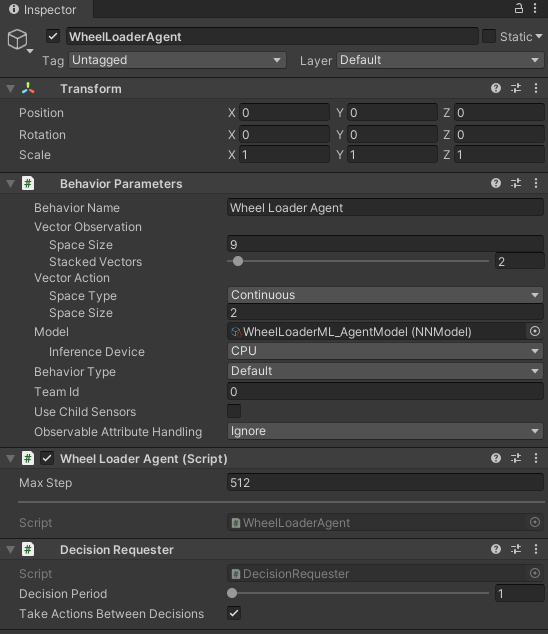
4.6.2. Create an Agent
The agent is created as an implementation of the ML-Agents base class Agent.
Create a new GameObject
Add a new Component and choose the script WheelLoaderAgent
Add a new Component and choose Decision Requester
Set the fields on the component as in:
There are three important methods that must be implemented in every agent script.
OnEpisodeBegin()- initializes and resets the agent and the environment each episode.CollectObservations(VectorSensor sensor)- collects the vector observations every time a decision is requested.OnActionRecieved(float[] vectorAction)- sets the action computed by the policy each time a decision is requested.
Each of these are described in more detail below.
4.6.3. Initialization and Resetting the Agent
Instead of importing the wheel loader prefab into the unity scene it is created at runtime by the Agent script. When a RL-training episode ends it is common to reset the agent as well as other things in the scene. If your agent is a simple system of bodies you might be able to easily reset the transforms, velocities etc. However, for more complicated models it is usually easier to completely remove them from the simulation and reinitialize them. The typical way to do this in AGXUnity is:
// Destroy the gameobject for the wheel loader.
DestroyImmediate( WheelLoaderGameObject );
// Manually call garbage collect. Important to avoid crashes.
AGXUnity.Simulation.Instance.Native.garbageCollect();
// Reinitiate the wheel loader object
WheelLoaderGameObject                     = Instantiate( WheelLoaderResource );
WheelLoaderGameObject.transform.position  = new Vector3( 40.0f, 0.07f, 1.79f );
WheelLoaderGameObject.transform.rotation  = Quaternion.Euler( -90, 0, 0 );
WheelLoader = WheelLoaderGameObject.AddComponent<AGXUnity.Model.WheelLoader>().GetInitialized<AGXUnity.Model.WheelLoader>();
foreach( var script in WheelLoaderGameObject.GetComponentsInChildren<AGXUnity.ScriptComponent>() )
  script.GetInitialized<AGXUnity.ScriptComponent>();
When training the Agent (wheel loader), it attempts to solve the task of driving towards the next target. The training
episode ends if the Agent; achieves the goal, is too far away from the goal or times out. At the start of each episode, the
OnEpisodeBegin() method is called to set-up the environment for a new episode. In this case we:
Check if the way points exists, if not, it creates a couple of random way points.
If we reached the final way point we call destroy on the wheel loader and the terrain and recreates them again.
Set the next active way point.
Before the first episode, the ML-Agents Academy is set to only step after the Simulation have stepped. By default the
ML-Agents Academy steps each FixedUpdate(). But since it is not required to step the Simulation
in FixedUpdate() it is safer to make sure the Academy steps in PostStepForward.
// Turn off automatic environment stepping
Academy.Instance.AutomaticSteppingEnabled = false;
// Make sure environment steps in simulation post.
Simulation.Instance.StepCallbacks.PostStepForward += Academy.Instance.EnvironmentStep;
4.6.4. Observing the Environment
The agent must observe the environment to make a decision. ML-Agents supports scalar observations collected in a feature vector and/or full
visual observations, i.e. camera renderings. In this example we use simple scalar observations since visual observations can often
leads to long training times. The agent must receive enough observations to be able to solve the task. The vector observation is collected
in CollectObservations(VectorSensor sensor) method. In this example we give the agent the:
Distance to the next way point
The direction to the next way point in local coordinates
How the wheel loader leans in world coordinates
Angle between wheel loaders forward direction and way points forward direction
Current speed of the wheel loader
The angle of the wheel loader waist hinge
The speed of the wheel loaders waist hinge
The current RPM of the engine
These observations are also stacked four times (set in the Behavior Parameters component).
4.6.5. Taking Actions and Assigning Rewards
When driving towards a way point the wheel loader must control the throttle and the steering. We have chosen to exclude every
other possible action (elevate, tilt, brake) since they are not required for the task.
The computed actions are received as an argument in the method OnActionReceived(float[] vectorAction). They are clamped
to appropriate ranges and set as control signals on the engine and steeringHinge.
We use a sparse reward function. The agent receives a constant negative reward of \(r_t = -0.0001\) for each time step it did not reach the way point. Thus, encouraging it to reach the way point fast. If the agent passes the goal way point it receives a reward that depends on the distance to the way point and how well the wheel loader is aligned towards the way points forward direction. The reward is defined as,
Where \(r_{pos}\) and \(r_{rot}\) is defined as,
and
Where \(d\) is the distance to the passed way point and \(f_{\text{w}}\) is forward direction for the wheel loader and \(f_{\text{p}}\) is forward direction of the passed way point, both in world coordinates.
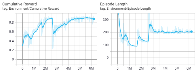
4.6.6. Training the Agent
After installing the ML-Agents python API you can train the agent using Soft-Actor-Critic (SAC) or Proximal-Policy-Optimization (PPO). For
a faster training session it is recommended to disable the deformable terrain game object and enable the box ground game object instead.
It is possible to start a training session that communicates directly with the Unity editor, enabling you to watch the agent to fail in
the beginning and continuously improving. Run the command mlagents-learn config.yaml --run-id=training_session and press play in
the Unity editor.
The file config.yaml specifies hyperparameters for the RL-algorithms. We have used:
behaviors:
  Wheel Loader Agent:
    trainer_type: ppo
    hyperparameters:
      batch_size: 2024
      buffer_size: 20240
      learning_rate: 1e-4
      beta: 1e-4
      epsilon: 0.2
      lambd: 0.95
      num_epoch: 3
      learning_rate_schedule: constant
    network_settings:
      normalize: true
      hidden_units: 64
      num_layers: 2
      vis_encode_type: simple
    reward_signals:
      extrinsic:
        gamma: 0.995
        strength: 1.0
    keep_checkpoints: 200
    checkpoint_interval: 100000
    max_steps: 2e7
    time_horizon: 512
    summary_freq: 10000

environment_parameters:
  wheel_loader_curriculum:
    curriculum:
      - name: close
        completion_criteria:
          measure: reward
          behavior: Wheel Loader Agent
          signal_smoothing: true
          min_lesson_length: 1000
          threshold: 0.85
        value:
          sampler_type: uniform
          sampler_parameters:
            min_value: 3.0
            max_value: 5.0
      - name: further
        completion_criteria:
          measure: reward
          behavior: Wheel Loader Agent
          signal_smoothing: true
          min_lesson_length: 1000
          threshold: 0.90
        value:
          sampler_type: uniform
          sampler_parameters:
            min_value: 4.5
            max_value: 8.0
      - name: furthest
        value:
          sampler_type: uniform
          sampler_parameters:
            min_value: 7.0
            max_value: 12.0
This is also an example of how to use curriculum learning in ML-Agents. We define three different lessons, which controls the possible distance to the next way point. Curriculum learning can greatly improve training times in sparse reward environments, by making the reward more likely in the beginning and then increasing the task difficulty gradually. It is very possible to improve these hyperparameters. For config options view the ML-Agents documentation.
Training in the editor can be quite slow. Alternatively, it is possible to build the unity project and specify the resulting executable as the environment with
the argument --env=<path to executable>. This avoids overhead from running the editor. For even faster training sessions add the arguments
--num-envs=N and --no-graphics, where the former starts N separate environments and the latter disables camera renderings. The command
can then be mlagents-learn config.yaml --env=BuildExample.exe --no-graphics --num-envs=2 --run-id=training_session. List all possible arguments with
mlagents-learn --help.
The training results is saved in the directory results/<run-id>. It is both tensorflow checkpoints that is used for resuming training sessions, and
exported <behavior-name>.nn model files. This is the final policy network saved in a format used by the Unity Inference Engine. In the editor it is possible
to use these trained models for inference, i.e. training of the policy do not continue, but the current policy is used to control the agent. Choose the file as
Model in the Behavior Parameters component for the relevant agent.
Finally it is possible to track the training progress using tensorboard. Run the command tensorboard --logdir=results, open a browser window and navigate to
localhost:6006.
4.7. ML-Agents Robot poking box controller
Note
AGX modules required to run example: Core
Download this example as a standalone package: AGXUnity_RobotML.unitypackage
In this ML-Agents example an agent is trained to control an industrial ABB robot. The goal is to move the robot’s end effector to a certain pose and remain there. The robot is controlled by setting the torque on each motor at each joint.
This example is trained using the ML-agent versions:
com.unity.ml-agents (C#) v.1.4.0.
mlagents (Python) v0.20.0.
mlagents-envs (Python) v0.20.0.
Communicator (C#/Python) v1.0.0.
4.7.1. The Learning Environment
The learning environment consist of the robot, the target box and a static ground. The goal for the robot is to match the target box transform with its tool tip. The robot aims for the middle of the box and to rotate the tip of the tool so that it aligns with the normal of the green side of the box. The simulation time step is 0.005 s and the length of each episode is 800 steps. The agent takes one decision each time step. When the episode ends, the target box is moved to a new random pose within a limited distance from the previous. The robot then aims for the new target pose from its current state, thus giving the agent experience of planning paths from different configurations. Every four episodes the state of the robot is also reset. The current agent was only trained on targets within a certain limited distance in front of the robot.
The robot is also reset if the tool tip collides with the robot. This ends the episode early, reducing the possible reward. Doing this speeds up the training in the early stages of training.
4.7.2. Action and Observations
The observation for the robot are
Current angle of each hinge joint
Current velocity of each hinge joint
The relative pose of the target compared to the tool tip
The tool tip pose relative to the robot
The tool tip velocity
This adds up to 30 scalars that are stacked for two time steps.
The action in each time step is the torque on each of the 6 motors for every hinge joint on the robot.
4.7.3. Reward
The agent is rewarded for being close to the target pose. The reward function shaped so that the agent starts to receive a small reward starting 0.7 meters away from the target and then increases exponentially.
The reward based on position is calculated as
The reward based on rotation is calculated as
where \(q\) is the quaternion between the tool and the target. The final reward is then
where \(c\) is a constant for scaling the reward.
4.8. Deck Crane
Note
AGX modules required to run example: Core, Wire
Download this example as a standalone package: AGXUnity_DeckCrane.unitypackage
The Deck Crane demonstrates the use of wires and some very useful constraints between rigid bodies. This scene is part of the video tutorial Modeling a crane with wires, available here: YouTube - Modeling a crane with wires . The Unity content starts at this timestamp.
The tutorial shows the workflow of modelling a complete crane system starting from a CAD model. It utilizes Algoryx Momentum for the modelling of the crane parts including dynamic properties such as joints, materials, rigid bodies and collision shapes.
4.9. Grasping Robot
Note
AGX modules required to run example: Core, Cable
Download this example as a standalone package: AGXUnity_GraspingRobot.unitypackage
This scene illustrate the use of DIRECT solver for frictional contacts. This allows for dry and robust contact friction. The robot is controlled using keyboard or a gamepad. This example uses the Input System package. For more information, see Section 4.5.11
The robot model has been created in Algoryx Momentum and imported into AGXUnity as a prefab.
4.9.1. Control using Gamepad
Right Stick Y - Moves the robot arm up/down
Left Stick X - Move the robot arm left/right
Left Stick Y - Move The robot arm in/out (from the base)
D-Pad (X/Y) - Controls the lower hinges which move the lower part of the robotic arm.
Button A/B - Open/Close Yaw
Right/Left Bumper - Rotate wrist left/right
4.9.2. Control using Keyboard
PageUp/Down - Moves the robot arm up/down
Left/Right - Move the robot arm left/right
Up/Down - Move The robot arm in/out (from the base)
W/S/A/D - Controls the lower hinges which move the lower part of the robotic arm.
Z/C - Open/Close Yaws
E/Q - Rotate wrist left/right
4.10. Articulated Robot
Note
AGX modules required to run example: Core
Download this example as a standalone package: AGXUnity_ArticulatedRobot.unitypackage
This scene demonstrates the Articulated Root component which enables the possibility to place Rigid Body instances in a hierarchical structure.
The model is an FBX model of a jointed robot system including two fingers for grasping.
4.10.1. Control using Gamepad
Left/Right trigger - open/close grasping device
Left/Right Shoulder - Rotate Hand
Left Horizontal - Rotate base
Left Vertical - Shoulder up/down
Right Vertical - Elbow
Right Horizontal - Wrist1
D-Pad vertical - Wrist2
D-Pad horizontal - Wrist3
4.10.2. Control using Keyboard
A/D - rotate base joint
S/W - rotate shoulder joint
Q/E - rotate elbow joint
O/P - rotate wrist1
K/L - rotate wrist2
N/M - rotate wrist3
V/B - rotate hand
X - close pincher
Z - open pincher
4.11. Excavator on terrain
Note
AGX modules required to run example: Core, Drivetrain, Tracks, Terrain
Download this example as a standalone package: AGXUnity_Excavator.unitypackage
This scene demonstrates an excavator with tracks operating on the AGX Dynamics Deformable Terrain.
The setup of the terrain is done in the same way as in the Wheel Loader on Terrain example.
For the setup of the input/steering we refer to the Wheel loader example
The control of the tracks are done via a drivetrain configuration including a combustion engine. For more information, see the implementation in the Engine class.
4.11.1. Control of camera
The camera is by default following the excavator using the LinkCamera.cs script. By pressing F1, the FPSCamera script is activated allowing for a free roaming camera.
F1 - Toggle FPSCamera
Left/Right - Move left/right
Up/Down - Move forward/backward
4.11.2. Control using Gamepad
Right Stick X - Boom up/down
Right Stick Y - Move bucket
Left Stick X - Swing left/right
Left Stick Y - Stick up/down
D-Pad (X/Y) - Drive forward/backward/left/right
4.11.3. Control using Keyboard
PageUp/Down - Boom up/down
Insert/Delete - Move bucket
T/U - Swing left/right
Home/End - Stick up/down
Up/Down - Forward/Backward
Left/Right - Turn Left/Right
4.11.4. Excavation measurements
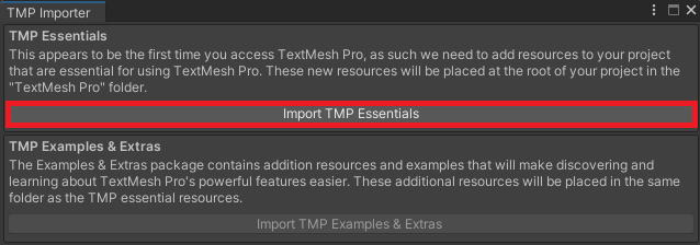
There is a second scene in the excavation example package which showcases how to measure the excavated mass and volume using the agxSensor library. This scene uses TextMeshPro and requires importing TextMeshPro Essentials. When opening the scene a window should open which prompts the user to import the required package.
4.12. Plotting
Note
AGX modules required to run example: Core
Download this example as a standalone package: AGXUnity_Plot.unitypackage
This scene demonstrates how to visualize data from the simulation with graphical plots.
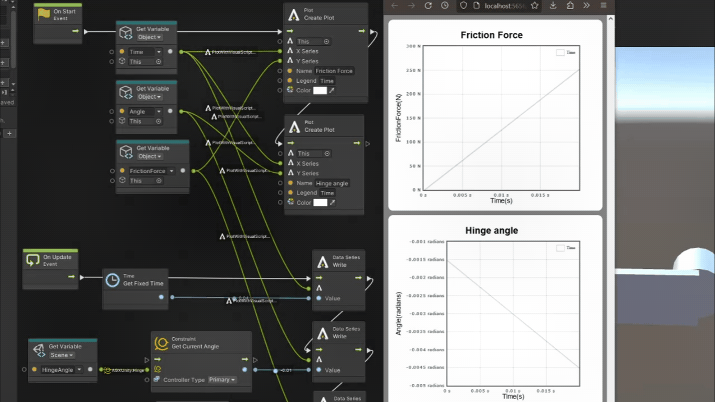
4.12.1. Plotting with Visual Scripting
Note
Unity Package required: Visual Scripting
Using the Unity Visual Scripting package, graphs can be set up and edited in a quick code-free way that offers great flexibility. The example package is set up to use this mode of plotting as-is.
Note
Please see the following guide for more details on the AGX Dynamics for Unity visual scripting: this guide
The graphs will be shown in the browser. The data can instead be written to a file on disk, which is also outlined in the guide
4.12.2. Plotting with Python server
Warning
This option is deprecated and might be removed in future updates
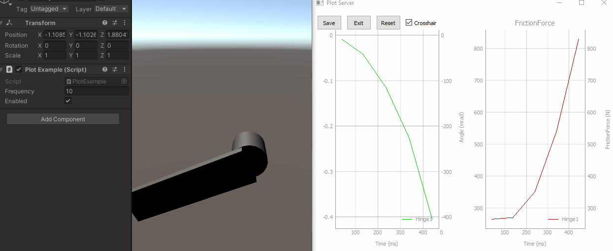
As an alternative to plotting with Visual Scripting, there is a Python based plot server. To enable this in the example,
deactivate the GameObject PlotWithVisualScripting and enable the component Plot Example on the GameObject PlotObjects.
4.12.2.1. Requirements
The plot server is written in Python (version 3) and requires a few additional modules to run.
It will listen to port 5555 by default (can be changed with an argument to the python script): start_plotServer.bat <portnumber>
To start the plot server on your local machine, double click the start_plotServer.bat:
Checking if Python3 is available...
Checking if Pip is available...
Checking for required Python modules...
Starting server...
Binding to port: 5555
Server started!
The script will verify that:
Python is available
the pip command (for checking python modules) is available
the required modules are available
If not, you will be informed to install the modules using the pip command:
pip install -r requirements.txt
4.12.2.2. Creating a plot session
The API for setting up a plot session is very simple. The SetupPlot() function below could be called from the Start() method
of a MonoBehaviour` class or similar. Plot windows and curves are identified via string names. So any string you use when you call
AddPlot() AddCurve() must be identical to when you call the AddData() method.
void SetupPlot()
{
   // Get a reference to the remote plot interface
   var plot = PythonPlot.PlotManager.Instance.Plot;

   // Important: Reset any previous plots in the plot server!!
   plot.Reset();

   // Add a Plot window with the title "Angle" and Time as x-axis and Angle as y-axis.
   plot.AddPlot("Angle", "Time", "s", "Angle", "rad");

   // Add a curve "Hinge1" to the plot named "Angle"
   plot.AddCurve("Angle", "Hinge1", PythonPlot.Color.Green());

   // Add another plot window with different units for the y-axis.
   plot.AddPlot("FrictionForce", "Time", "s", "FrictionForce", "N");
   plot.AddCurve("FrictionForce", "Hinge1", PythonPlot.Color.Red());
}
Next, to send data to the remote server the method AddData() should be called as often as there is new data. In the example below, the
UpdatePlot() function could be called from the Update() or FixedUpdate() method of a MonoBehaviour class.
void UpdatePlot()
{
   var plot = PythonPlot.PlotManager.Instance.Plot;
   var angleData = getTheAngle();
   var forceData = getTheForce();

   // Send data to the server identified with the "Angle" + "Hinge1"
   plot.AddData("Angle", "Hinge1", Time.time, angleData);

   // Send data with some force, identified with "FrictionForce" + "Hinge1"
   plotAddData("FrictionForce", "Hinge1", forceData);
}
4.12.2.3. Frequency
By default all data submitted using the AddData() method will be sent to the remote server. This could cause latency issues.
The frequency by which data is submitted can be set with the Frequency attribute. This will prune all data that is sent with higher frequency.
Note
Each dataset, identified with the title + curve parameters to the AddData() method will have its own timer to measure frequency.
var plot = PythonPlot.PlotManager.Instance.Plot;
plot.Frequency = 10; // Send data with 10 hz update rate.
4.12.2.4. Setting server address and port
If you want to run the plot server on a different computer (default is localhost), you can specify this _before_ accessing the PlotManager:
// Set the port and the address before accessing the Instance.
PythonPlot.PlotManager.Address = "127.0.0.1";
PythonPlot.PlotManager.Port = 5555;

var plot = PythonPlot.PlotManager.Instance.Plot;
// Setup your plot
4.13. Conveyor belt
Note
AGX modules required to run example: Core
Download this example as a standalone package: AGXUnity_ConveyorBelt.unitypackage
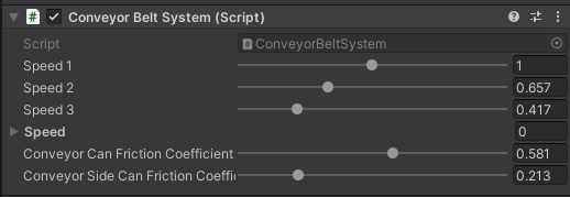
This example demonstrates how to use the surface velocity feature of Shapes.
By selecting the ConveyorBeltSystem in the hierarchy the speed of each lane as well as the friction between the can/conveyor and can/side can be controlled:
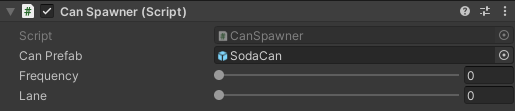
If the game object CanSpawner is selected, the rate by which cans are created can be controlled. In addition, the lane where the cans are being spawned can be changed.
4.14. Twisted cables
Note
AGX modules required to run example: Core
Download this example as a standalone package: AGXUnity_TwistedCables.unitypackage
This scene demonstrates the use of the cable model in a scenario where they will collide and interact due to twisting and bending. The cables are created in a C# script and are attached between the two disks. One of the disks is controlled using a rotational/translational constraint (CylindricalJoint) A motor is enabled for both the rotational and the translational degree of freedom which allows for rotation (twisting cables) and a linear motion (slacking cables). Current speed, the torque applied by the rotational part of the motor and the current cable stiffness is displayed in the window.
By changing the overall stiffness of the cable, they can be made very stiff (steel bars) or very soft.
This example also uses the Cable Damage component to visualize the normal forces applied to the various segments of the cable.
4.14.1. Control using Keyboard
Note
This example is using the legacy input UnityEngine.Input which will throw exceptions if the new Input System package is
installed and enabled. It’s possible to have both legacy and new input enabled by selecting Both under
Edit -> Project Settings... -> Player -> [Configuration] Active Input Handling.
Left/Right - Move disk left/right
Up/Down - Change rotation speed of the disk
Home - Stop movement/rotation
Page up/down - Increase/decrease cable stiffness
4.15. Car drivetrain
Note
AGX modules required to run example: Core, Drivetrain, Tires
Download this example as a standalone package: AGXUnity_Car.unitypackage
This example features the finished scene built in Tutorial 5: Modelling a car with drivetrain and ackermann steering which is part of the AGXUnity YouTube tutorial series.
The car’s drivetrain is built in a C# script and this example showcases how to interact with the built drivetrain directly to gear up and accelerate the vehicle as well as how to read back data such as the current gear and the speed of the wheels from the drivetrain.
Additionally this example shows how Ackermann steering can be setup to steer the vehicle.
4.15.1. Control using Keyboard
Up/Down - Drive forward/backward
Left/Right - Turn left/right
Page up/down - Gear up/down
4.16. Ocean simulation
Note
AGX modules required to run example: Core, Hydrodynamics
Download this example as a standalone package: AGXUnity_Ocean.unitypackage
This example showcases how to dynamically set a water geometry using an external wave simulation. In this example, the open source project FFT-Ocean is used to generate the waves.
The glue which generates and updates the water geometry is located in the WaterHeightField.cs script. The main component of this script is to create and maintain a Height Field which contains the height data read from the wave data.
4.17. Terrain manipulation
Note
AGX modules required to run example: Core, Terrain
Download this example as a standalone package: AGXUnity_TerrainManipulation.unitypackage
This scene demonstrates how to use the terrain API to get and set the terrain heights. This example performs a ray-terrain intersection test to find the intersection point where the line shot from the camera through the mouse cursor intersects the terrain. The terrain heights in the region surrounding the intersection point is then retrieved and changed depending on the selected manipulation operation being performed. After the heights have been modified, they are written back into the terrain. The effect is a type of painting on the terrain using the cursor.
4.17.1. Controls
Left mouse button - Raise the terrain at the cursor position
Right mouse button - Lower the terrain at the cursor position
Middle mouse button - Smooth the terrain at the cursor position
R - Reset the heights in the terrain to the initial heights
G -
Debug.Logthe height of the terrain at the cursor position
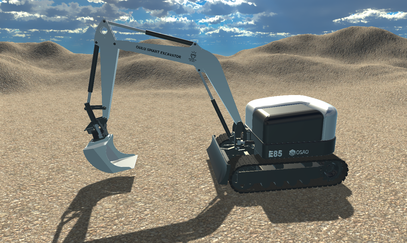
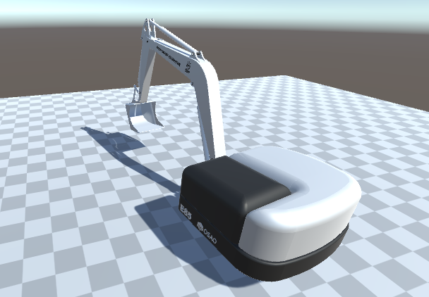
4.18. E85 excavator
Note
AGX modules required to run example: Core, Tracks, Terrain
Download this example as a standalone package: AGXUnity_ExcavatorE85.unitypackage
This scene demonstrates an E85 excavator with tracks operating on the AGX Dynamics Deformable Terrain, similar to the Excavator on terrain. The differences between the scenes are that in this scene, the tracks are not powered by a drivetrain and the excavator has a few extra parts to control, for example the blade in front of the tracks.
Just as for Excavator on terrain, setup of the terrain and the input system, check Wheel Loader on Terrain example and Wheel loader example.
4.18.1. Control of camera
The camera is by default following the excavator using three different cameras that you can switch between to get different angles, set up in the ExcavatorE85CameraHandler script. By pressing F1, the ExcavatorE85FPSCamera script is activated allowing for a free roaming camera. This is similar to the FPSCamera in the Excavator on terrain example, but with slightly different controls.
F1 - Toggle FPSCamera
A/D - Move left/right
W/S - Move forward/backward
Mouse - Camera look direction
Space - Switch camera
4.18.2. Control using Gamepad
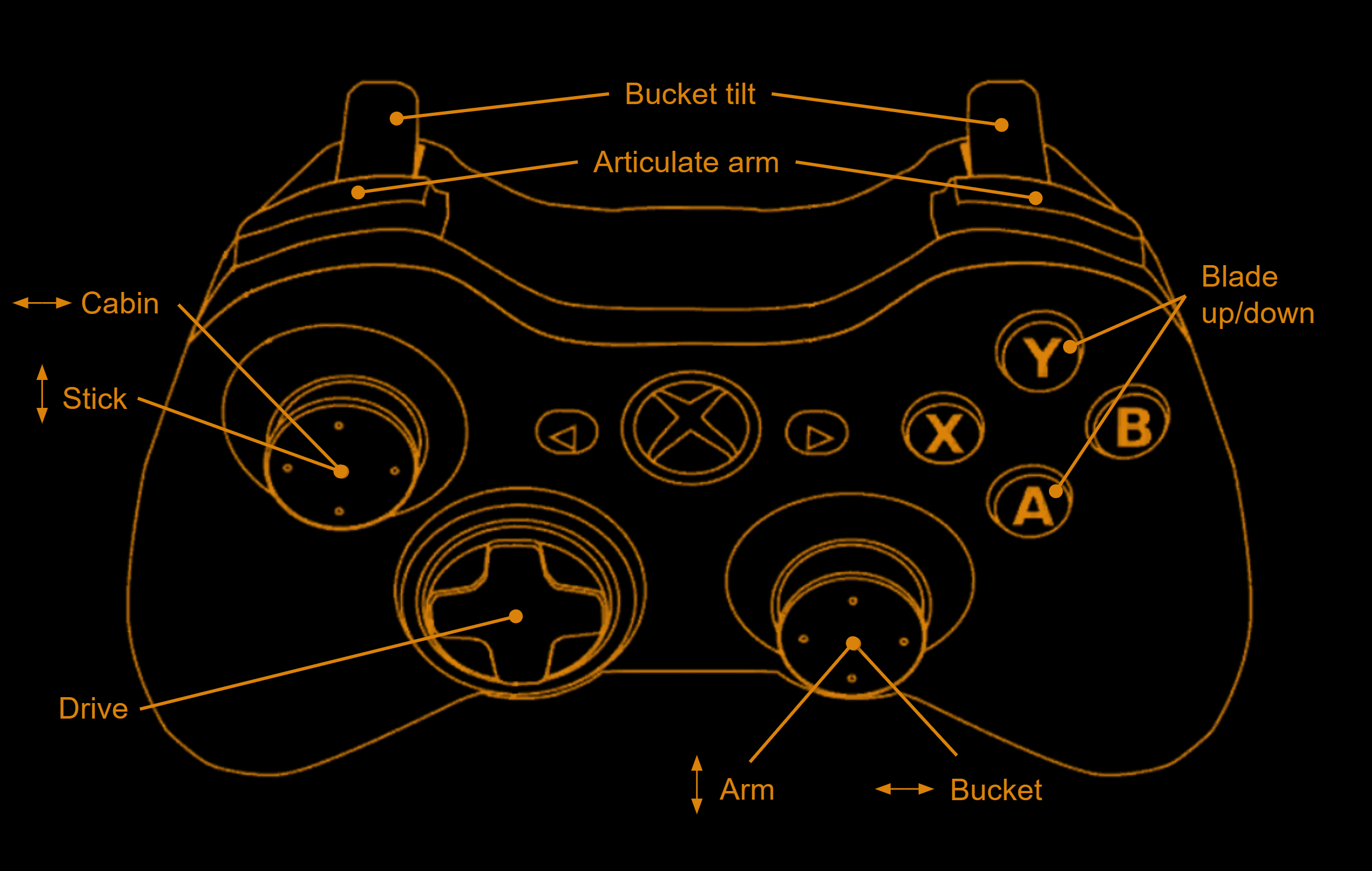
4.18.3. Control using Keyboard
Page Up/Down - Right track forward/backward
Home/End - Left track forward/backward
Left/Right arrow - Cabin left/right
Up/Down arrow - Blade up/down
R/F - Arm up/down
T/G - Stick up/down
Y/H - Stick up/down
V/B - Arm articulation left/right
N/M - Bucket tilt left/right
Z - Reset scene
4.19. Polybag demo
Note
AGX modules required to run example: Core
Warning
This example is a prototype for simulating flexible objects such as polybags. This model is a work in progress and will not be supported in the future. The purpose of this model is for evaluation only.
Download this example as a standalone package: AGXUnity_Polybag.unitypackage
This demo showcases how to simulate deformable polybags in AGXUnity using lumped element modelling.
Each polybag consists of a set of rigid bodies with corresponding collisions shapes which are connected by
6DOF-Constraints (LockJoints) where the flexibility of the polybag as a whole is controlled by modifying the
compliance of the constraints. Polybags are implemented in the Polybag.cs script which exposes a number of properties:
Property |
Description |
|---|---|
resolution |
Specifies the resolution of the model. Keep this at LOW for now. It has a large effect on performance as a higher resolution will create more rigid bodies, shapes and constraints. |
length |
Specifies the length of the bag (m). |
width |
Specifies the width of the bag (m). |
height |
Specifies the height of the bag (m). |
compressibility |
Higher value indicates a softer bag in the compression aspect. |
bendability |
Higher value indicates a softer bag in terms of bending. |
mass |
Total mass of the bag (kg). |
renderMaterial |
The render material used for the polybag. |
material |
The physical Shape Material of the polybag. |
polybagMesh |
The 3D mesh asset that should define the bag. |
useContactReduction |
If true, a contact reduction will be performed between the bag and other objects. For other friction model solvers than ITERATIVE this can have a huge positive performance impact. |
In the demo scene, these properties are set on the PolybagEmitter class instead of on the polybags directly.
The emitter creates and initializes bags automatically at set intervals at the emitters position.
These bags are transported along a simple surface velocity conveyor belt which applies a velocity constraint at each contact point.
The logic for the conveyor belt is contained in the SurfaceVelocity.cs script which additionally applies a texture offset to
the render material to visualize belt movement.
At the end of the conveyor belt there is a sensor which removes the polybags that comes into contact with the sink geometry.
This sink is implemented using Contact Callbacks in the ObjectSink.cs script.
The visual mesh is update each frame based on the underlying simulated deformable mesh. While this is a quite expensive operation, the updating is offloaded onto separate threads using the Unity Job System, yielding a substantial performance increase. Thus, this example also showcases how to utilize the Job System when using data from large vectors in agx.
Note
As this demo uses Unity’s Burst compiler to speed up it’s jobs, the com.unity.burst package is required to run this demo.
4.19.1. Limitations
Currently the dimensions (length, with, height) of a polybag is quite limited. We have only tested with the current scenario. We know that making the size in Length < Width will generate invalid geometries, causing the simulation to behave poorly.
We know that using thin meshes will cause problems due to very small volumes for collision geometries.
Additionally, there is no plasticity for this model, meaning that the model will strive to move back into its initial state after deformation.
4.20. Bed Truck
Note
AGX modules required to run example: Core, Terrain, Drivetrain, Tires
Download this example as a standalone package: AGXUnity_BedTruck.unitypackage
This example showcases some of terrain features which can be used to optimize a terrain scene. Specifically, this example makes use of the Deformable Terrain Pager as well as the Movable Terrain.
The Deformable Terrain Pager is used to reduce the size of the terrain that is being simulated for any given time step. The pager is setup to track the position of the Wheel Loader shovel as well as the main body of the Bed Truck. This means that as the bed truck moves, new parts of the terrain will be loaded and old parts will be unloaded as needed.
The Movable Terrain is used to reduce the amount of terrain particles in the scene. The Bed Truck bed has a terrain component which replaces the bottom box. This allows for particles to merge into the bed which vastly reduces the computational load of the scene, and allows for large amounts of material to be moved without incurring the performance cost of thousands of particles.
Using the Movable Terrain does require a method for converting the terrain back to dynamic particles as well. In this example this is done by adding a Soil failure volumes which converts part of the terrain to dynamic particles when the bed is tipped. While this method of converting the terrain is not physically sound, it is easy to implement and is sufficient to showcase the movable terrain in this example.
4.20.1. Control using Gamepad
D-Pad Right - Swap selected machine
Right/Left Trigger - Drive forward/backward
Left Joystick - Turn left/right
Right Joystick - Tip bucket or truck bed
D-Pad Up/Down - Gear up/down (Bed Truck only)
4.20.2. Control using Keyboard
Tab - Swap selected machine
W/S - Drive forward/backward
A/D - Turn left/right
Left/Right - Tip bucket or truck bed
Q/E - Gear up/down (Bed Truck only)
4.21. Sample Asset Package
Download this example as a standalone package: AGXUnity_SampleAssets.unitypackage
One of the main considerations of building stable and accurate simulations is to find proper values for the various parameters available to tweak. This can be a daunting task and requires a lot of proper measurements and calibration and can be quite a hurdle for setting up new project.
The purpose of this example is to provide a reasonable set of default assets which can be used for experimenting with different parameters in new projects.
4.21.1. Disclaimer
The physical properties presented in this package are collected from a variety of different sources, many of which disagree on particular values for the same properties of the same material (or material pair). Additionally many of the properties here depend on the particular characteristics of the specific material being used (smooth or rough, temperature etc.) or conditions in which a collision occur (dry or greased, impact velocity, etc.).
This is to say that this collection of materials should only be used as a “getting started” to get a feel for the various parameters available in AGX. For more serious applications, materials and contact materials have to be explicitly measured in a controlled environment.
4.21.2. Contents
The following section outlines the content contained in this sample package. For all of the tables in the section, the following legend applies:
*: Entries marked with “*” use values from the AGX material library which is included with the AGX installation.
**: Entries marked with “**” are calculated based on the individual material properties. For restitution, the formula \(r = \sqrt{r_1*r_2}\) is used (individual material restitutions not presented in table). For Young’s modulus, the formula \((y_1 * y_2)\div (y_1 + y_2)\) is used. (See the AGX Material Documentation) for more information.)
?: Entries marked with “?” have no real basis in any measurements and are simply filled in based on “feel”.
4.21.2.1. Shape Materials
The following table lists the Shape Material assets in the asset pack.
Material Name |
Density (kg/m^3) |
Wire Bend YM (GPa) |
Wire Stretch YM (GPa) |
|---|---|---|---|
Aluminum |
2700* |
69 [1] |
69 [1] |
Asphalt |
2300* |
1.9 [2] |
1.9 [2] |
Concrete |
2400* |
17 [1] |
17 [1] |
Hemp Rope |
1400 [3] |
35 [1] |
0.1? |
Nylon |
1140 [4] |
3 [1] |
1? |
Rubber |
940* |
0.05* |
0.05* |
Steel |
7800* |
98* |
98* |
Stone |
2700* |
60 [5] |
60 [5] |
Wood |
520* |
11.9 [6] |
11.9 [6] |
4.21.2.2. Terrain Materials
The following terrain materials have been internally calibrated by Algoryx and should roughly approximate the corresponding material properties when used by a terrain component:
Dirt
Gravel
Sand
Snow (experimental)
For brevity, these parameters are not tabulated here, please refer to the actual assets for parameter values.
Note
Each of these the terrain materials have corresponding Shape Material. These materials does not contain any meaningful material info and should only be used as material handles for contact materials. See the Internal Material Handles property on the Deformable Terrain component.
4.21.2.3. Contact Materials
The following table lists the Contact Material assets in the asset pack. Most of these are ported directly from the AGX material library. Note that there are multiple shape material pairs for which there is no contact material.
Material 1 |
Material 2 |
Friction coefficient |
Restitution |
Young’s Modulus |
|---|---|---|---|---|
Aluminum |
Aluminum |
1.05 [7] |
0.1** |
6.9e8 [1] |
Aluminum |
Rubber |
1.0* |
0.95* |
6.66e7* |
Aluminum |
Steel |
0.61* |
0.4* |
5.74e10* |
Aluminum |
Stone |
0.38* |
0.63* |
3.24e10* |
Asphalt |
Concrete |
0.55* |
0.61* |
6.93e8* |
Asphalt |
Rubber |
0.7* |
0.42* |
6.1e7* |
Asphalt |
Stone |
0.4* |
0.6* |
7.12e8* |
Asphalt |
Wood |
0.4* |
0.6* |
6.81e8* |
Concrete |
Concrete |
0.8* |
0.85* |
8.7e9* |
Concrete |
Rubber |
1.0* |
0.4* |
6.64e7* |
Concrete |
Steel |
0.57* |
0.84* |
1.61e10* |
Concrete |
Stone |
0.575* |
0.6* |
6.1e9* |
Concrete |
Wood |
0.62* |
0.71* |
7.17e9* |
Hemp Rope |
Steel |
0.5 [7] |
0.3? |
2.98e10** |
Hemp Rope |
Wood |
0.5 [7] |
0.3? |
8.9e9** |
Nylon |
Nylon |
0.2 [7] |
0.35? |
3e9 [1] |
Nylon |
Steel |
0.4 [7] |
0.45? |
2.96e9** |
Rubber |
Rubber |
1.16* |
0.4* |
3.33e7* |
Rubber |
Steel |
1.0* |
0.4* |
6.66e7* |
Rubber |
Stone |
1.0* |
0.4* |
6.66e7* |
Rubber |
Wood |
0.825* |
0.4* |
6.63e7* |
Steel |
Steel |
0.225* |
0.78* |
1.1e11* |
Steel |
Stone |
0.4* |
0.82* |
4.43e10* |
Steel |
Wood |
0.55* |
0.61* |
1.16e10* |
Stone |
Stone |
0.85* |
0.83* |
2.77e10* |
Stone |
Wood |
0.7* |
0.65* |
1.0e10* |
Wood |
Wood |
0.45* |
0.6* |
5.1e9* |
4.21.2.4. Contact Materials for terrain applications
The following table lists the Contact Material assets corresponding to terrain materials in the asset pack.
Note
The Shape Material corresponding to the terrain material has to be added as an Internal Material Handle to relevant terrains for these contact materials to work.
Terrain Material |
Material 2 |
Friction Coefficient |
Restitution |
Young’s Modulus |
|---|---|---|---|---|
Dirt |
Concrete |
0.3 [8] |
0.0** |
6.5e6** |
Dirt |
Rubber |
0.65 [9] |
0.0** |
5.8e6** |
Dirt |
Steel |
0.5 [10] |
0.0** |
6.5e6** |
Gravel |
Concrete |
0.55 [11] |
0.65** |
4.6e6** |
Gravel |
Rubber |
0.6 [9] |
0.45** |
4.2e6** |
Gravel |
Steel |
0.4 [11] |
0.62** |
4.6e6** |
Sand |
Concrete |
0.4 [11] |
0.0** |
4.5e6** |
Sand |
Rubber |
0.6 [9] |
0.0** |
5.8e6** |
Sand |
Steel |
0.3 [11] |
0.0** |
4.5e6** |
Snow |
Aluminum |
0.4 [7] |
0.0** |
6.5e6** |
Snow |
Nylon |
0.4 [7] |
0.0** |
6.5e6** |
Snow |
Rubber |
0.2 [9] |
0.0** |
5.8e6** |
Snow |
Steel |
0.2 [12] |
0.0** |
6.5e6** |
4.21.3. Showcase scenes
Included in the asset pack are a few sample scenes which are meant to display the differences between the included assets.
4.21.3.1. Material Showcase
The material showcase scene (AGXUnity_SampleAssets.unity) showcases the frictional and restitutional properties of the Contact Material assets in the asset pack as well as the visual materials corresponding to the Shape Material assets.
Spheres of each contact material is dropped on boxes of each material to showcase restitution of each contact material pair.
To showcase the friction, boxes of each materials is placed on a ground plate of each material and the ground plate is rotated, causing the boxes to start sliding depending on the frictional properties of the contact material.
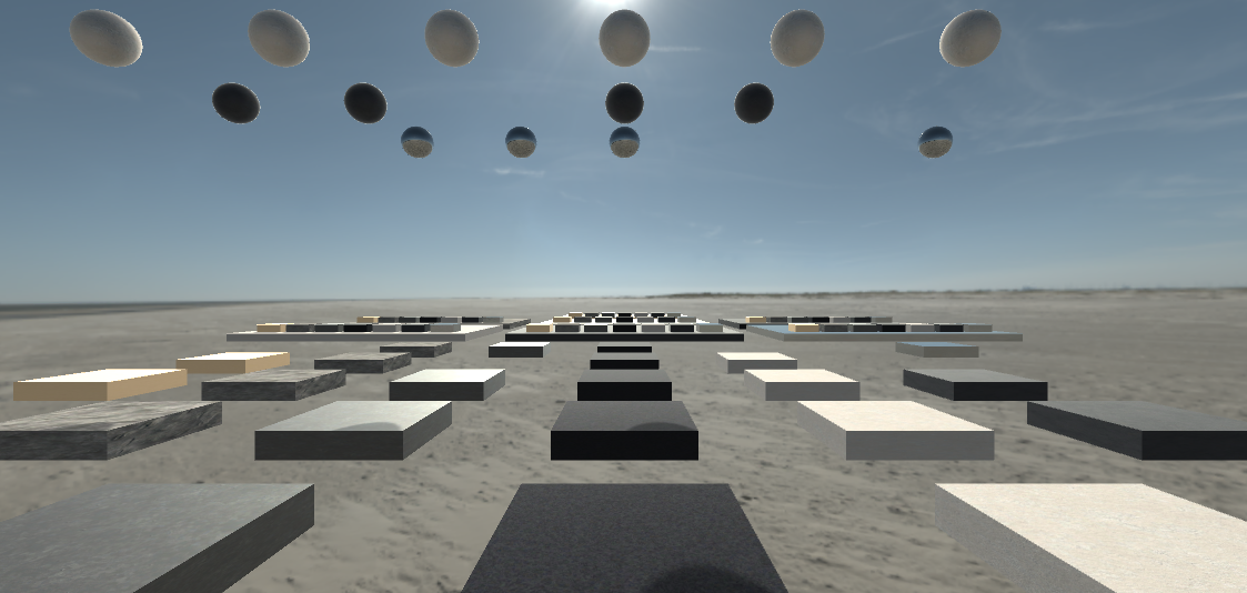
Initial state of the material showcase scenes.
4.21.3.2. Wire Showcase
The wire showcase scene showcases the wire bending and stretching stiffnesses of the wire Shape Material assets in the asset pack as well as the visual materials corresponding to those.
Note
The rendering materials use a custom shader to properly render scaled cables as described in Rendering the wire. Please refer to the section, Custom AGXUnity rendering materials, for information about using these materials in URP or HDRP projects.
To showcase the bending stiffness of each wire material, a wire is dropped over a cylinder which will cause some bending due to gravity. For stiffer materials this bending will be smaller.
To showcase the stretching stiffness, a ball is connected to on end of the wire and the wire is dropped over a cylinder. The weight of the ball will attempt to stretch the wire.
Note
The weight of the connected ball is set to 20 000 kg to exaggerate the stretching stiffness.
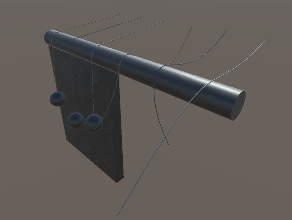
Relaxed state of the wire showcase.
4.21.3.3. Terrain Showcase
The terrain showcase scene showcases how different Deformable Terrain Material asset properties impact the excavation, merging, and granular simulations of the included Deformable Terrain Material assets. Additionally it showcases how to render different granular materials for different terrains.
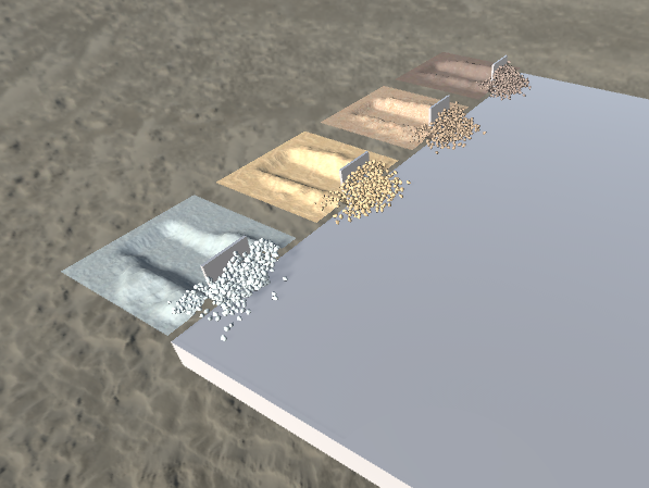
Terrain showcase scene
4.22. Using ROS2 in AGXUnity
Download this example as a standalone package: AGXUnity_ROS2.unitypackage
While the AGXUnity plugin itself does not contain Unity components for publishing or subscribing to ROS2 topics, this functionality is available through the AGX C# scripting API. This example showcases a simple scene contains two scripts, one that publishes the image rendered by a Unity camera to a topic and another that subscribes to the same topic and updates the main texture of a plane’s material.
The resulting scene is a camera and screen setup. Notably though, since the communication goes through A ROS2 topic, it is possible for external applications to subscribe to the topic and receive the rendered image alongside the in-project subscriber.
4.22.1. Data transfer performance considerations
Since the data being sent is a rendered image, certain considerations have to be taken into account to avoid extreme performance drops.
First off, the data is read back from a RenderTexture on the GPU. This is an inherently slow operation since it requires CPU/GPU synchronization. For this reason, this example uses Unity’s AsyncGPUReadback API. This does, however, mean that the image that is published, is not necessarily the same as the one that was rendered the current frame, but might be an older image.
Secondly, actually transforming the data into the proper format for sending over the ROS2 API might incur some overhead. In this case, since the data is an array of many bytes, iterating over the byte array and inserting into the C#-wrapped vector causes the performance of the whole project to drop unacceptably. For this reason, the Set/Get methods are used to avoid the overhead of iterating a long array. Please refer to the AGX Dynamics User Manual for more information about handling long arrays.
4.23. Inhomogeneous Terrain
Download this example as a standalone package: AGXUnity_InhomogeneousTerrain.unitypackage
This example showcases how to use the TerrainMaterialPatch component to use different physics materials in different parts of the terrain. In the example, a pile of sand as well as a patch of ice has been modelled using TerrainMaterialPatch components. Additionally, the example uses the TerrainPatchRenderer component to visualize the different terrain materials.
The controls in the example is the same as in Wheel Loader on Terrain.
4.24. OpenPLX Tutorials
Download this example as a standalone package: AGXUnity_OpenPLX.unitypackage
Every AGX installation comes with a set of tutorials which are intended to teach the basics of using OpenPLX to model simulations effectively. These are intended to be used with the agxViewer application that is packaged with the AGX installation but given that AGXUnity has OpenPLX import capabilities, these can be easily modified to work with AGXUnity.
This section will outline the changes needed to adapt the tutorials for use in AGXUnity but in general the process for creating the OpenPLX models will be the same as in the AGX version of the tutorials.
4.24.1. OpenPLX model library
The package also includes a models folder with reusable OpenPLX models that can be imported directly
or used as references when building custom OpenPLX assets:
AlgoryxLunarCruiser- Lunar cruiser model with drivetrain variants and Python examples.BeachBuggy- Wheeled vehicle model with reusable suspension and drivetrain components.BoxTruck- Box truck model used by several tutorial scenes.CAT_D10- Bulldozer model assets used by the advanced bulldozer tutorial.KomatsuHM400- Articulated dump truck model with angle-control and linear-actuator variants, scenarios, and signal interfaces.Panda- Panda robot assets and variants used by the URDF robot tutorials.TrafficCone- Simple traffic cone model used by lidar and vehicle examples.VehicleWithSteering- Compact steering vehicle model for control examples.
The model library follows the folder conventions documented in models/README.md in the example package.
4.24.2. General changes
Given that agxViewer uses python to load the OpenPLX models and to control the imported model, the following changes are required for all tutorials:
In AGXUnity, all models are imported using a custom ScriptedImporter which means that the import step is no longer necessary as part of the script. Instead the imported asset simply has to be added to a Unity scene.
Unity uses C# for scripting instead of python so the scripts have to be ported to C#. This has been done and the ported scripts are included in the example package. Since the script no longer loads the model the script instead has to be added to the loaded model after it has been added to the scene.
An additional change is required to read and propagate input to the OpenPLX model via OpenPLX signals. This is handled via
a utility script named InputActionMapper.cs located in the root example package directory which allows mappings to
be created from Unity InputActions to OpenPLX Signals. This utility is used in each tutorial where user input is required
and a simple mapping is sufficient.
All tutorials reference external files for visual/collision meshes or .agx imports. These files are located under <Example Root>/data
and the Example includes an editor script which sets the AGX_DATA_DIR environment variable to this directory to allow the OpenPLX importer
to find these external files. This script is located under the <Example Root>/Editor directory. This does however mean that runtime import does not work for these
files as the importer will be unable to locate these external data files unless the same environment variable is set explicitly.
4.24.3. Tutorial 1 - Introduction to OpenPLX: Boxtruck
AGX version of the tutorial: Intro to OpenPLX - Boxtruck Tutorial 01

This tutorial basically works out of the box after applying the general changes by creating a control script as well as a scene with the imported model.
4.24.4. Tutorial 2 - Introduction to Automatic Assembly
AGX version of the tutorial: Tutorial 02 - Introduction to automatic assembly
The only notable change for this tutorial is that the ObserverFrame debugging is enabled by default in AGXUnity. To manually disable/enable this feature, check out the MateConnector Mapping section.
4.24.5. Tutorial 3 - URDF Robot
AGX version of the tutorial Tutorial 03 - Urdf Robot Modeling

This tutorial works out of the box with the general changes applied.
4.24.6. Tutorial 4 - Signal Interface
AGX version of the tutorial Tutorial 04 — Signal Interface

This example illustrates how to use signal interfaces defined in OpenPLX. Signal interfaces are useful as they allow a model author to easily communicate which signals are relevant for downstream users of the model. This example is almost identical to Tutorial 1 but with two notable differences:
When mapping inputs to signals, the signal endpoints are found via a call to the
SignalInterface.FindInputmethod with the signal interface name as the parameter instead of finding the input using the fully qualified name of the signal via theOpenPLXSignals.FindInputTargetmethod.The controller script additionally displays the cached output signals for the outputs specified in the signal interface. This illustrates how to iterate the interface and how to query the endpoints for metadata.
4.24.7. Tutorial 5 - Lidar Autobrake
AGX version of the tutorial Tutorial 05 - Lidar Autobrake System

This tutorial is currently incomplete as AGXUnity does not yet support OpenPLX lidar signals. Instead, the controller script in this tutorial adds it’s own LidarOutput to enable reading the scan points generated by the lidar. However, since the value sent to the motors have to be modified depending on the Autobrake engage status, the input mapping utility is not used in this tutorial.
Finally, the lidar mapping does not automatically add a point cloud renderer component so this component has been added to the scene object instead.
4.24.8. Tutorial 6 - Wheeled Vehicle
AGX version of the tutorial Tutorial 06 - Vehicle with Wheels
This tutorial only requires the general changes to work with AGXUnity but note that the input mapping used in this tutorial is different as the input signals are interpolated over time instead of immediately switching from no signal to full signal.
4.24.9. Tutorial 7 - IMU
AGX version of the tutorial Tutorial 07 - IMU
This example is a work-in-progress as AGXUnity does not yet support reading sensor signals.
4.24.10. Tutorial 8 - URDF Robot Control
AGX version of the tutorial Tutorial 08 - Urdf Robot Control
This example is the one that requires the most changes due to the controller itself making heavy use of the AGX API rather than using signals for control. This means that the entire inverse dynamics controller needs to be ported to C# and that the AGXUnity API has to be used instead to connect everything.
The PandaController.cs script does all of the heavy lifting here but some parts in particular is worth pointing out as they give insight into how to
use the OpenPLX API even when direct calls to the AGX API is required:
First off, the controller makes heavy use of the
OpenPLXRoot.FindMappedObjectmethod in the form ofpanda.FindMappedObject( <openplx name> ).GetComponent<...>(). This is a common pattern to get the component that a specific OpenPLX model was mapped onto when the mapped type is known.Secondly, the controller uses
panda.Native.getObject( "panda" ).getObject( $"panda_joint{i+1}" ).getNumber( "initial_angle" )to get the initial pose for the robot. This is an example of how to retrieve values directly from the OpenPLX file. Another example where this can be used is to store custom data that the mapper does not necessarily care about, e.g. the model name or ID of a specific vehicle.Finally, the controller also exemplifies how to use the signal endpoint wrappers directly. That is, by fetching them via the OpenPLXSignals.FindOutputSource/FindInputTarget methods and reading/sending signals via the
GetValueandSendSignalmethods respectively.
Regarding the tool replacement part of the original tutorial: this can be done by changing the Imported Model import option of the panda_move.openplx
as described in Import options.
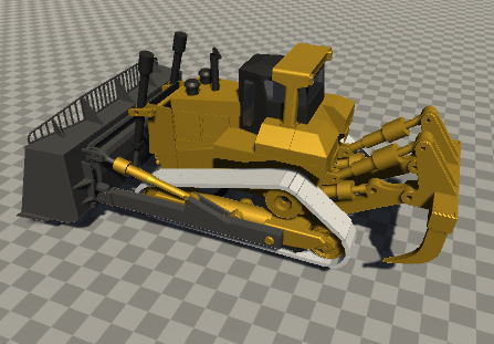
4.24.11. Advanced Tutorial 1 - Bulldozer
AGX version of the tutorial OpenPLX Tutorial - Importing and Enhancing a Bulldozer Model from .agx File
The following is a list of changes and general notes for applicable steps:
Step 2: Terrains in OpenPLX use Movable terrain due to limitations in how Unity terrains can be used. This can cause performance issues for larger terrains.
Step 3: When splitting OpenPLX models into different files, the resulting models are sometimes missing references that are set when actually using the model. This will cause import errors when Unity attempts to import the incomplete models. To avoid these errors, we can instruct the importer to skip importing these files by selecting the files in the project asset view and toggling Skip Import in the inspector.
4.24.12. Advanced Tutorial 2 - Build a Heavy Machine Bundle
AGX version of the tutorial Tutorial - Heavy Machine Bundle
This tutorial works as intended right away but as for the bulldozer tutorial, it can be nice to disable import of the incomplete models in the constructed bundle to avoid getting import errors on reimports. When downloading the finished example, these should be pre-disabled.
4.24.13. Advanced Tutorial 3 - Excavator Arm - Use the Heavy Machine Bundle
AGX version of the tutorial Tutorial 05 - Excavator Arm - using the heavy machine bundle
The following is a list of changes and general notes for applicable steps:
Step 1: As agxViewer is no longer used, the
--addBundlePathargument is no longer available. The corresponding method to add a bundle dependency in AGXUnity is to add the bundle path underAGXUnity > Settings > OpenPLX Settings > Additional Bundle Directorieswhich will then be added to the OpenPLX import context for subsequent asset imports.